EGU Short course code (part 2)

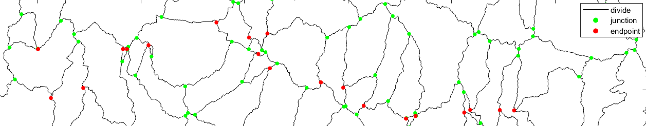
The second part of our EGU Short Course on Analyzing transient landscapes using TopoToolbox focused on the analysis of drainage divides using @DIVIDEobj, a numerical class to store, analyze and visualize drainage divides. The data for the course can be downloaded here. Below, you’ll find Dirk’s commented code that shows how to analyze drainage divides in the Parachute Creek.

% Working with divide objects (DIVIDEobj)
load('alos_preprocessed.mat')

% We'll work on the entire DEM and derive the stream network
FA = flowacc(FD);
S = STREAMobj(FD,FA>1000);
D0 = DIVIDEobj(FD,S,'verbose',true);

% as it seems to take a long time to obtain the divide network, we aborted
% the process and make the stream object smaller by choosing a larger
% drainage area threshold
S = STREAMobj(FD,FA>10000);

% we can also shrink the stream object by segments using the function
% "modify". Let's do that too and have a look at the output
plot(S)
hold on
S = modify(S,'streamorder','>1');
plot(S)

% now derive the divide object again and look at the results
D0 = DIVIDEobj(FD,S,'verbose',true);
plot(D0,'color','k')
% the next thing is to order the divide segments in the network
D = divorder(D0,'topo');

% let's examine the results in the context of the DEM and the stream
% network
imageschs(DEM)
hold on
plot(S,'w','linewidth',1)
plot(D,'color','k')

% The divide network is defined by the drainage basins, which are sensitive
% to truncation of rivers like the Colorado River. To avoid spurious
% divides along the edges of the DEM, we use the function "cleanedges"
D = cleanedges(D,FD);

imageschs(DEM)
hold on
plot(S,'w','linewidth',1)
plot(D,'color','k')


%% across divide metrics
% We'll look at some across-divide metrics and see what we want to use in
% conjunction with the divide network

% 1. Hillslope angle
G = gradient8(DEM,'deg');

% inspect results
imagesc(G), hold on
plot(S,'w','linewidth',1)
plot(D,'color','k')

% any sampling of the underlying GRIDobj and mapping values to the divide
% object is best done with the pixels on opposite side of the divides. To
% get a sense of these locations, we briefly get the points and plot them
% in the active figure
[~,~,pix,qix] = getvalue(D,G);
[x1,y1] = ind2coord(DEM,pix);
[x2,y2] = ind2coord(DEM,qix);
scatter([x1;x2],[y1;y2],20,'ko','filled')

% by zooming in on the divides, we see that local slope angles close to the
% divide do not seem to be the best representation of the overall 
% morphology of the divide. Let's choose other metrics, where the values on
% the pixels next to the divides appear more meaningful


% 2. Hillslope relief
DZ = vertdistance2stream(FD,S,DEM);
% inspect results
imagesc(DZ), hold on
plot(S,'w','linewidth',1)
plot(D,'color','k')

% the pixels close to the divide seem to better caputre the entire
% hillslope relief - that's good. But some neighboring drainages seem to 
% have high while others have low relief values, which can be explained by
% the limited extent of the stream network, which sometimes reaches the
% plateau surface but sometimes not. To avoid these issues, we simply use a
% more extensive stream network.

% the actual value depends on what we consider a meaningful threshold value
% of the drainage area. Here, we choose a small value (100 pixel), but it 
% is intersting to compare the results using different values.
S2 = STREAMobj(FD,FA>100);
DZ = vertdistance2stream(FD,S2,DEM);

% inspect results
imagesc(DZ), hold on
plot(S2,'w','linewidth',1)
plot(D,'color','k')


% 3. Chi: using the same more extensive stream network, we finally compute
% chi values and map these from the stream network to the divide pixels.
% Note this can be equally done with any other property of the stream
% network, like ksn, for example.
c = chitransform(S2,FA);
C = mapfromnal(FD,S2,c);

% inspect results
imagesc(C), hold on
plot(S2,'w','linewidth',1)
plot(D,'color','k')

% Note that the truncation of streams in our DEM, especially rivers like
% the Colorado that have a large upstream drainage area affects our chi
% values and thus the results. 


%% sampling across divide metrics 
% we've seen before that we can sample any GRIDobj using the function
% "getvalues"
[p,q,pix,qix] = getvalue(D,DZ);
dz = abs(diff([p,q],1,2));
imageschs(DEM,[],'colormap',[.9 .9 .9],'colorbar',false)
hold on
plotc(D,dz,'caxis',[0 300],'limit',[1000 inf])
colorbar
title('Across-divide difference in hillslope relief (m)')


% the function "asymmetry" does the same, but goes a step further and
% collects the observations from the individual pixel-wise divide edges
% and computes average values for divide segments that are limited by 
% junctions and/or endpoints. It also takes the magnitude and direction of
% the asymmetry values to compute a vector for each divide segment that can
% be used to display an arrow, for example, indicating the direction of the
% divide migration.

% note that we overwrite the stream object "S" here, because we copied the
% code lines below simply from the explanation (help) of the function 
% "asymmetry". As this is the end of the code in this exercise, we don't
% care...

[MS,S] = asymmetry(D,DZ);
for i = 1 : length(S)
    S(i).length = max(getdistance(S(i).x,S(i).y));
end
imageschs(DEM,[],'colormap',[.9 .9 .9],'colorbar',false);
%imageschs(DEM,gradient8(DEM,'deg'),'caxis',[0 45]) % with slope as background
hold on
plotc(D,vertcat(S.rho),'caxis',[0 0.5],'limit',[1000 inf])
colormap(gca,flipud(pink))
axis image
hc = colorbar;
hc.Label.String = 'Divide asymmetry index';
hold on
ix = [MS.dist]>1000; % & [MS.rho]>0;
f = [S.length]./1e3;
quiver([MS(ix).X],[MS(ix).Y],[MS(ix).u].*f(ix),[MS(ix).v].*f(ix),2,...
    'color','r','linewidth',1)
title('Drainage divide asymmetry and direction of lower hillslope relief')