EGU Short course code (part 1)

The first part of our EGU Short Course on Analyzing transient landscapes using TopoToolbox focused on the analysis of knickpoints using the numerical object PPS. The data can be downloaded here. Below, you’ll find the commented code that shows how to analyze and model the distribution of knickpoints in the Parachute Creek using point pattern analysis.

load('alos_preprocessed.mat')
imageschs(DEM)
hold on
plot(S,'w')

%% Pick outlet manually
% S = modify(S,'interactive','outlet');
% alternatively, you can also use
% extractconncomps(S)
% and pick the Parachute Creek basin

% pick outlet automatically (12654533)
ix = 12645284;
S  = modify(S,'upstreamto',ix); 

%% Knickpoints
[zs,kp] = knickpointfinder(S,DEM,'split',false,...
                                 'tol',150,'plot',true);

%% Create a PPS object
P = PPS(S,'PP',kp.IXgrid,'z',DEM);

%% Calculate chi
A = flowacc(FD);
c = chitransform(S,A,"mn",0.45);

%% Using rhohat

% Rhohat implements a nonparametric model of covariate dependence. 
r = rhohat(P,'cov',c);

%% Why would you use rhohat instead of ksdensity
% Rhohat returns spatial densities and is not a probability density
% function
P2 = generatepoints(P,'n',4,'distance',c);
ksdensity(getmarks(P2,c),'bandwidth',100)
rhohat(P2,'cov',c,'bandwidth',50)

%% Parametric model of knickpoint locations

% While rhohat is able to reveal the dependency structure, it doesn't
% provide a good model of the dispersion of knickpoint chi values

% A parametric model for a set of knickpoints is a second-order loglinear
% polynomial model (it's like a Gaussian distribution, but is not a
% probability density function but a function for the spatial density
% conditional on the variable chi).

[mdl,int,mx,sigmamx] = fitloglinear(P,c,'model','poly2');
figure
ploteffects(P,mdl);
xline(mx)
xline([mx+sigmamx mx-sigmamx],':')

% mx is the "best" estimate for the location of knickpoints in chi space
figure
plot(P)
PH = getlocation(S,mx,'value',c,'output','PPS');
hold on
plotpoints(PH,'color','b')

%% Now let's explore the function mnoptimkp

% mnoptimkp tries to find an optimal mn-ratio. If we set the option
% 'method', to 'deviance', then the output argument is a structure array
% that contains estimates of K and tau. In order, for K and tau to make
% sense, we need to set the parameter 't', the time since onset of
% incision.

results = mnoptimkp(P,FD,'method','deviance','t',8e6,'sigmat',1e6);
plotc(S,results.tau)
PH = getlocation(S,8e6,'value',results.tau,'output','PPS');
hold on
plotpoints(PH,'color','r')
hold off

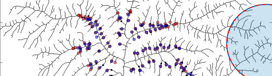
%% With drainage area loss

ixA0 = 14545684;
results2 = mnoptimkp(P,FD,'method','deviance','t',8e6,'sigmat',1e6,...
    'inletix',ixA0,'inletA0',1e6,'optimizemn',false,'mn0',0.4);

PH2 = getlocation(S,8e6,'value',results2.tau,'output','PPS');

plot(P)
hold on
plotpoints(PH,'color','r')
plotpoints(PH2,'color','b')

% sidelength of lost area
sl = sqrt(results2.addA_m2);
[x,y] = ind2coord(DEM,ixA0);
radius = sqrt(results2.addA_m2/pi);
h = drawcircle('Center',[x,y],'Radius',radius,'StripeColor','red',...
    'InteractionsAllowed','none');